인공지능 및 기계학습 개론 2(7.4~7.6) 정리
Dobby-HJ
·2023. 10. 2. 19:07
7.4 Bayes Ball Algorithm
Typical Local Structures
- Common parent
- Fixing “alarm” decouples “JohnCalls” and “MarryCalls”
- $J \bot M|A$ → A에 대한 정보가 있을 때, $J$와 $M$은 independent하다.
- $P(J, M|A) = P(J|A)P(M|A)$
- Cascading
- Fixing “alarm” decouples “Buglary” and “MaryCalls”
- $B\bot M|A$ → A에 대한 정보가 있을 때 $B$와 $M$은 independent하다.
- $P(M|B,A) = P(M|A)$

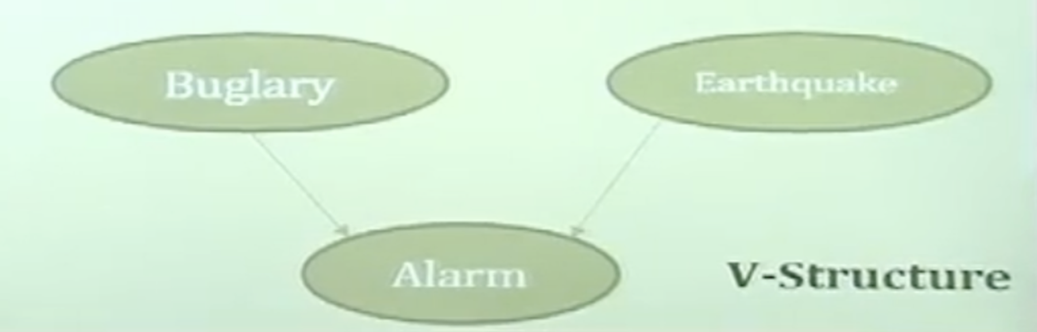
- V-Structure
- Fixing “alarm” couples “Buglary” and “Earthquake”
- $\sim (B\bot E|A)$
- $P(B,E,A) = P(B)P(E)P(A|B,E)$
- Any algorithm for complex graph?
Bayes Ball Algorithm
- Purpose : checking $X_A \bot X_B|X_c$
→ 특정 Random Variable $X_c$가 주어졌을 때 또다른 Random Variable $X_A, X_B$가 independent할 지 판정하는 알고리즘. Ball로써 graphical 하게 이해할 수 있음. - 쉽게 생각하면 정보가 given인 상태에서는 색을 칠하고 아니라면 색을 칠하지 않음.
이후에 칠해져 있는 부분은 통과하지 못하는 부분으로 인식해서 흐름도를 그렸을 때 연결되지 않으면 그것은 independent한 관계임.- Shade all nodes in $X_c$
- Place balls at each node in $X_A$
- Let the ball rolling on the graph by Bayes ball rules
- Then, ask whether there is any ball reaching $X_B$
Exercies of Bayes Ball Algorithm
-
- $P(A|lanket, B) = P(A|blanket)$
$Blanket = {\text{parents}, \text{childern}, \text{children's other parents}}$ - Blanket과 condition할 수 있다면, Blanket 외부의 것과는 무조건 independent하다.
- Markov Blanket
- $P(A|lanket, B) = P(A|blanket)$

- D-Seperation
- $X$ is d-separated(directly-separated) from $Z$ givn $Y$ if we cannot send a ball from any node in $X$ to any node in $Z$ using the Bayes ball algorithm
7.5 Factorization of Bayesian networks
Factorization of Bayesian Network
- Factorization theorem
- Given a Bayesian network
- The most general form of the probability distribution
- that is consistent with the probabilitic independencies encoded in the network
- Factorizes according to the node given its parents
- $P(x)= \Pi_i P(X_i|X_{\pi_i})$
- $X_{\pi_i}$ is the set of parent nodes of $X_i$
- The most general form
- What are the not-mose general form???
- More discussions of d-separation, not going to be in this classroom
- $P(X_1, X_2, X_3)=P(X1∣X2,X3)P(X2∣X3)P(X3)$
→ 원래는 이렇게 구해야하는데, $P(x)= \Pi_i P(X_i|X_{\pi_i})$ 여기 식에 의해 parents에 의한 조건부 확률로 구분할 수 있음.

Plate Notation
- Let’s consider a certain Gaussian model
- Many $Xs$
- Depend upon the same parameter
- Mean and Variance
- Independent between $Xs$
- 단순히 여러 Random Variable들을 상자로 묶어서 표현(Notation)함.
- Dealing with many random variables
- Simplify the graphical notation with a box
- Works like a for-loop
- $P(D|\theta) = P(X_1, \dots X_N|\mu, \sigma)\=\Pi_N(P(X_1|\mu,\sigma)$
- Naive assumption
- Likelihood function
- $L(\theta|D) = P(D|\theta)$

7.6 Inference Question on Bayesian network
Infernce Question 1: Likelihood
- Given a set of evidence, what is the likelihood of the evidence set?
- $X = {X_1, \dots, X_N}$ : all random variables → 전체 확률 변수
- $X_V = {X_{k+1}, \dots, X_N}$ : evidence variables → 관측한 확률 변수 혹은 알아보고자 하는 확률 변수
- $X_H = X - X_V = {X_1, \dots, X_k}$: hidden variabels → 명시적으로 다루지는 않지만 hidden 되어서, 현재의 causality 속에서는 감안을 해줘야 하는 내용이다.
- 여기서 "hidden variables"라는 용어는 그 변수들이 관측되지 않았거나, 모델링 과정에서 직접적으로 다루지 않지만, 그래도 중요한 역할을 하는 변수들을 의미합니다. 예를 들어, 어떤 병의 발병 원인을 연구할 때, 직접적인 원인 외에도 다른 숨겨진 요인들이 있을 수 있습니다. 이러한 숨겨진 요인들은 직접적으로 관측되지 않지만, 병의 발병을 이해하거나 예측하기 위해 고려해야 합니다.
- "현재의 causality 속에서는 감안을 해줘야 하는 내용"이라는 부분은 이 숨겨진 변수들이 원인과 결과의 관계, 즉 인과 관계(causality)에 영향을 줄 수 있기 때문에, 분석이나 모델링 과정에서 이러한 변수들을 고려해야 한다는 것을 의미합니다.
- General form
- $P(x_V)= \sum_{X_H}P(X_H, X_V)\
= \sum_{x_1}\dots\sum_{x_k}P(x_1\dots x_k, x_V)$ - Likelihood of $x_V$
- $P(x_V)= \sum_{X_H}P(X_H, X_V)\
Infernce Question 2: Conditional Probability
- $P(A|B=true, MC = true)$일 때의 확률 값은 근사적으로 얼마일까?에 대한 의문을 해석하는 부분.
- Given a set of evidence, what is the conditional probability of interested hidden variables?
- $X_H = {Y, Z}$
- $Y$ : interested hidden variables
- $Z$ : uninterested hidden variables
- $X_H = {Y, Z}$
- General form
- $P(Y|x_V) = \sum_ZP(Y, Z = z|x_v)\
= \sum_Z\cfrac{P(Y, Z, x_V}{P(x_v)}\
= \sum_Z \cfrac{P(Y, Z, x_V)}{\sum_{y, z}P(Y=y, Z = z, x_v)}$- 첫 번째 식에서 $Z$가 나오는 이유는 현재 우리가 구하고자 하는 값은 $Z$와 연관이 없기 때문에 marginalize가 가능함. 이를 full joint한 것.
- 이렇게 full joint를 구했으면 2번째 줄의 수식이 가볍게 나온다.
전체 input 확률 변수들의 full joint에 대한 확률을 normalize constant인 $P(x_V)$로 나눠준다. - 마지막의 $P(x_v)$에 대해서 $P(x_V)= \sum_{X_H}P(X_H, X_V) = \sum_{x_1}\dots\sum_{x_k}P(x_1\dots x_k, x_V)$를 유도했었으므로 이를 동일하게 작성하면 된다. 여기서 2개로 확장되는 것은 $X_H = {X_y, X_z}$이기 때문.
- Conditional probability of $Y$ given $x_v$
- $P(Y|x_V) = \sum_ZP(Y, Z = z|x_v)\
Inference Question 3: Most Probable Assignment
- Given a set of evidence, what is the most probable assignment, or explanation given the evidence?
- Some variables of interests
- Need to utilize the inference question 2
- Conditional probability
- Maximum a posteriori configuration of $Y$
- Applications of a posteriori
- Prediction
- $B,E$ → $A$
→ 그래프 구조에 의해서 $B, E$가 주어졌을 때는 $A$는 어떻게 될까요? 하고 “예측”하는 것.
$P(A|B,E)$를 구하는 것.
- $B,E$ → $A$
- Diagnosis
- $A$ → $B, E$
→ $A$가 주어졌을 때, $B, E$의 assignment는 어떻게 될까?
$P(B,E|A)$를 구하는 것.
- $A$ → $B, E$
- Prediction
질문
- $P(X_1 | X_2, X_3)$라는 식에서 $x_1\bot x_3 | x_2$라는 가정이 첨가되면 원래 4개의 parameter가 필요했지만 이제 2개의 parameter가 된다고 해. 그 이유는 $P(X_1 | X_2)$로 변화하기 때문이야.이렇게 되면, 원래는 $X_1$의 각 값에 대해 $X_2$와 $X_3$의 모든 조합에 대한 조건부 확률을 지정해야 했지만, 이제는 $X_1$의 각 값에 대해 $X_2$의 값만 고려하면 됩니다. 따라서 필요한 매개변수의 수가 크게 줄어들게 됩니다.
- 예를 들어, $X_1$, $X_2$, $X_3$ 각각이 2개의 값만 가질 수 있다고 가정하면, 원래는 4개의 조건부 확률 값을 지정해야 했습니다. 하지만 $x_1 \bot x_3 | x_2$ 가정이 추가되면, 2개의 조건부 확률 값만 지정하면 됩니다. 이렇게 매개변수의 수가 줄어들게 됩니다.
- $x_1 \bot x_3 | x_2$는 $x_2$가 주어졌을 때 $x_1$과 $x_3$이 독립적이라는 것을 의미합니다. 이 가정이 추가되면, $P(X_1 | X_2, X_3)$를 $P(X_1 | X_2)$로 단순화할 수 있습니다.
'DeepLearning > 인공지능 개론' 카테고리의 다른 글
| 인공지능 및 기계학습 개론 2(8.4~8.5) 정리 (5) | 2023.10.15 |
|---|---|
| 인공지능 및 기계학습 개론 2(8.1~8.3) 정리 (1) | 2023.10.14 |
| 인공지능 및 기계학습 개론 2(7.7~7.9) 정리 (1) | 2023.10.09 |
| 인공지능 및 기계학습 개론 2(7.1~7.3) 정리 (0) | 2023.10.01 |